Introduction

So you might be wondering - what is a characteristic function? What are iverson brackets? And what am I doing here?

A characteristic function (or indicator function) of a set is defined via the following: Given \(Y\subseteq X\), \(\chi_{Y}:X\to\left\{0,1\right\}\), where \(\chi_{Y}(x)=\begin{cases} 1 & x\in Y \\ 0 & x\not\in Y \end{cases}\). We can also denote this function \(1_{Y}\) (with a bold face 1 - that format isn't available using MathJax). Essentially, this is a function that gives a \(1\) output when we have some variable \(x\) in the given subset \(Y\), and \(0\) otherwise.

This function is particularly useful when you want a representation for checking for variables in an arbitrary domain or set - and not strictly in a single variable either. We can also have several variations of this function in two variables that performs the same way - with that being said, the implementation is up to the person. The techniques I'll discuss in this post can be applied to several variables, but will become more difficult to manage as the number of restrictions increases.

Finally, we also have the Iverson bracket. Iverson brackets denote a similar, but slightly more generalised idea. We denote it like so: \(\left[S\right]\), where \(\left[S\right]=\begin{cases} 1 & S\ \textrm{true} \\ 0 & \textrm{else} \end{cases}\), given some sentence/proposition \(S\). In our case, the indicator or characteristic function of a set given above can be denoted using this notation as \(\left[x\in Y\right]\).

General form

The Iverson bracket, in general, cannot be written in a form that does not use itself in the definition, as far as is known. With that being said, it's not a necessarily (in most cases it's not at all) continuous function. That does not mean, however, that special cases, such as the characteristic function, cannot be written in a form that's more recognisable.

In fact, a good number of characteristic functions can be written in terms of signum. But first we must introduce the concept of turning inequalities into equalities. We'll do this as follows, sticking to the reals:

Let \(\omega:X\to\mathbb{R}\), \(\omega(x)\) denote the function such that \(\omega(x)=0\iff x\in Y\), where \(Y\subseteq X\). By consequence, then, \(\omega(x)\neq 0\implies x\not\in Y\).

We thus have an analogue for our characteristic function, in terms of our function \(\omega\):

\[ \begin{align} \chi_Y(x) &= \begin{cases} 1 & x\in Y \\ 0 & x\not\in Y \end{cases} \\ &= \begin{cases} 1 & \omega(x)=0 \\ 0 & \omega(x)\neq 0 \end{cases} \\ & = 1-\begin{cases} 1 & \omega(x)>0 \\ 0 & \omega(x)=0 \\ 1 & \omega(x)<0 \end{cases} \\ & = 1-\left|\operatorname{sgn}(\omega(x))\right| \end{align}\]

The idea now is that we find some function, \(\omega(x)\), such that this is satisfied. We know of some techniques already, but this post will go into them in more depth. The idea, in general though, is that we take a given set and convert its representation into an equality of some kind.

Interestingly, also, if we multiply both sides of our representation for the characteristic function by \(|\omega(x)|\) we get that \(|\omega(x)|\chi_{Y}(x)=0\). This always holds true, if \(\omega(x)\) exists. Just a nice little observation I guess.

Set operation analogues

Union

Given that we have some function \(\omega(x)=0\implies x\in Y\), it stands to reason that one of the most fundamental functional ideas/laws when solving equations pops out to us immediately as a union analogue: the null factor law. If \(\omega(x)=\omega_{1}(x)\omega_{2}(x)\dots\omega_{n}(x)\), then \(\omega(x)=0\implies\omega_{1}(x)=0\lor\omega_{2}(x)=0,\lor\dots,\lor\omega_{n}(x)=0\). Given that these functions are also functional analogues to sets also, it's only reasonable that they, like \(\omega(x)\), represent desired subsets for which \(x\) makes this expression true.

Complement

One method for finding the complement is checking all other possible values for a given function \(\omega(x)\) and then constructing another function, say, \(\omega'(x)\), accounting for these values in the same way we've done otherwise. For example, \((x>a)'=x\leq a\). As we'll see below, the former is given by \(\operatorname{sgn}(x-a)-1\) and the latter can be given by \((x-a)(\operatorname{sgn}(x-a)+1)\).

Alternatively, we know that for some condition \(x\in Y\iff \omega(x)=0\) so then the complement of this is \(x\not\in Y\iff \omega(x)\neq 0\). This is equivalent to \(|\omega(x)|>0\), or \(\operatorname{sgn}(|\omega(x)|)-1=0\), as we'll see using the techniques below.

We can also use this to write intersections. Take the following for example: Begin with \(\lnot(x\in A\land x\in B)\implies (x\not\in A \lor x\not\in B)\), by De Morgan's law. Consequently, this is equivalent to \([x\in A][x\in B]=0\). Finally, we'll complement to obtain the result:

\[ \operatorname{sgn}(|[x\in A][x\in B]|)-1=0\iff x\in A\land x\in B\]

This can be simplified because our two Iverson brackets take values in \(\left\{0,1\right\}\) (can be verified via piecewise form):

\[ [x\in A][x\in B]-1=0\iff x\in A\land x\in B\]

For those well-versed in Iverson bracket notation, this is also a consequence of \([P\land Q]=[P][Q]\). Furthermore, this can be verified by translating our original logical expression to our functional analogue and going from there instead.

Intersection

Alternatively to the above method, let us consider the following: For some \(f:U\to\mathbb{R},\ g:V\to\mathbb{R}\), then, for example:

1. \((f+g)(x)=f(x)+g(x)=y\), for some \(x\in U\cap V\).
2. \((f\cdot g)(x)=f(x)g(x)=y\), for some \(x\in U\cap V\).

There are, of course, more operations on these functions that have the same restrictions. But for simplicity, we'll limit ourselves to these.

The issue with intersections of functions with this method is that once we've combined functions like this, we need to check 'uniqueness' of our solution. In the functional cases I give below, this is fairly straightforward; the functions are piecewise and the values can be checked by solving for the actual form of our piecewise function and their respective domains. For example, \(\operatorname{sgn}(a)+\operatorname{sgn}(b)=2\) is uniquely true when \(a>0\) and \(b>0\).

Function analogues

We already know of a few functions that will allow us to represent certain conditions as equalities (and by extension, functions).

Infinite intervals

Both signum and absolute value functions reign here.

\[ \operatorname{sgn}(x-a)-1=0 \iff x\in\left(a,\infty\right)\ (x>a)\]

\[ \operatorname{sgn}(x-a)+1=0 \iff x\in\left(-\infty,a\right)\ (x<a)\]

To construct half-closed intervals, we union with a root of \(x-a\) and obtain:

\[ |x-a|-(x-a)=0 \iff x\in\left[a,\infty\right)\ (x\geq a)\]

\[ |x-a|+(x-a)=0 \iff x\in\left(-\infty,a\right]\ (x\leq a)\]

\(x\neq a\) is given by the complement of \(x-a=0\).

Discrete sets

Potentially the simplest sets, these can be represented by roots of polynomials (or series...).

Given some finite or countably infinite set, we can represent some set \(S\) by:

\[ \omega(x)=\prod_{s\in S}(x-s)=0\iff x\in S\]

Other useful functions that can represent countably infinite discrete sets are (some) periodic functions, such as the mod function, as well as trigonometric functions.

Notably, this is just a special case of the null factor law, or union analogue, as given above.

For integers and non-integers, notice we can just take the product as above over the positive and negative integers, as well as zero. An alternative, however is this relation:

\[ \left\lceil x\right\rceil-\left\lfloor x\right\rfloor=\begin{cases} 0 & x\in Z \\ 1 & x\not\in Z \end{cases}\]

Continuous finite intervals

From the floor function, we know that \(\left\lfloor x\right\rfloor=0\iff x\in\left[0,1\right)\). Therefore, given some \(b>a\):

\[ \omega(x)=\left\lfloor\frac{x-a}{b-a}\right\rfloor=0\iff x\in\left[a,b\right)\]

From the ceiling function, we know that \(\left\lceil x\right\rceil =1\iff x\in\left(0,1\right]\). Therefore, given some \(b>a\):

\[ \omega(x)=\left\lceil\frac{x-a}{b-a}\right\rceil-1=0\iff x\in\left(a,b\right]\]

For an open interval, there are several main ways to represent it. Given the above and our knowledge of intersections, we can represent it as the following:

\[ \omega(x)=\left\lfloor\frac{x-a}{b-a}\right\rfloor+\left\lceil\frac{x-a}{b-a}\right\rceil-1=0\iff x\in\left(a,b\right)\]

Alternatively, we can use our knowledge of the absolute value, triangle inequality, and signum. Given \(a<x<b\), we have \((a-b)<2x-(a+b)<(b-a)\implies |2x-(a+b)|<b-a\). From here, we deduce that:

\[ \omega(x)=\operatorname{sgn}(|2x-a-b|+a-b|)+1=0\iff x\in\left(a,b\right)\]

For \(\left[a,b\right]\), we can construct this in multiple ways; the easiest being the union of a root and a ceiling, or union of a root and a floor function.

Consequences

You remember how we are able to product closed shapes with one equation? Well, one consequence of this is that we are able to produce functions which determine whether a given point lies within a given shape or region. The examples are given below:

The code for these are incredibly simple; my implementation is 4 lines per shape, 6 lines to render.

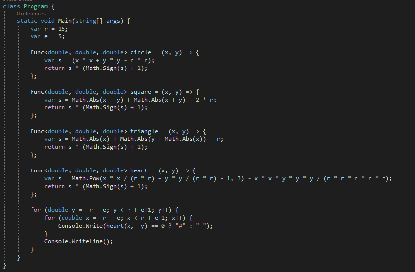
Let \(\omega_S(x)\) denote the relation for which the 'outline' of the shape is given. For example, a circle's equation is given by \(x^2+y^2-1\). Per the techniques as above, we can determine if \(\omega_S(x)\leq 0\) by \(\omega_S(x)(\operatorname{sgn}(\omega_S(x))+1)=0\).

Obviously this doesn't lend itself to cleanliness in terms of code, but it is a neat little trick. It also provides a technique to produce an explicit equation for mapping to a boolean analogue (in our case, 0 or 1) for basically anything we can give an equation for.